AI Daytrading
December 2024
Stage 1: Data
After searching many low-cost APIs for loading historical training data, I found Twelvedata to have the best access to markets. A simple script was sufficient to repeatedly load the data and save it to a CSV.
Data fetching

API_URL = "https://api.twelvedata.com/time_series"
SYMBOL, INTERVAL, OUTPUTSIZE, NUM_CALLS, ORDER = "NVDA", "1min", 5000, 10, "desc"
OUTPUT_CSV = f"data/{SYMBOL}_{INTERVAL}_{round(OUTPUTSIZE*NUM_CALLS/1000)}k.csv"
SLEEP_INTERVAL, all_data, last_end_date = 6.5, [], None

for call in range(1, NUM_CALLS + 1):
    print(f"API Call {call}/{NUM_CALLS}")
    params = {"symbol": SYMBOL, "interval": INTERVAL, "outputsize": OUTPUTSIZE, "order": ORDER, "apikey": API_KEY, "format": "JSON"}
    if last_end_date: params["end_date"] = last_end_date
    try:
        r = requests.get(API_URL, params=params); r.raise_for_status()
        data = r.json()
        df = pd.DataFrame(data["values"])
    except requests.exceptions.RequestException as e:
        print(f"Request Exception: {e}"); break

    df['datetime'] = pd.to_datetime(df['datetime'])
    df[['open', 'high', 'low', 'close', 'volume']] = df[['open', 'high', 'low', 'close', 'volume']].apply(pd.to_numeric, errors='coerce')

    df.dropna(inplace=True)
    all_data.append(df)
    last_end_date = (df['datetime'].min() - timedelta(minutes=1)).isoformat()
    print(f"Fetched {len(df)} data points.")
    print(f"Next call will use end_date <= {last_end_date}")
    time.sleep(SLEEP_INTERVAL)

combined_df = pd.concat(all_data, ignore_index=True)
combined_df.drop_duplicates(subset=['datetime'], inplace=True)
combined_df.sort_values('datetime', inplace=True)
combined_df.reset_index(drop=True, inplace=True)
combined_df.to_csv(OUTPUT_CSV, index=False)
print(f"Data saved to {OUTPUT_CSV}")
print(f"Total data points fetched: {len(combined_df)}")
In total, I loaded roughly 2.8 million minutes worth of data from tech stocks and cryptocurrencies. Using just a single consumer-grade GPU made it impractical to train on much more than this. Whilst trading in the live markets, fast data is the only way to retain a profitable strategy, for which I would need a different source.
Stage 2: LSTM approach
My starting approach was a simple LSTM layout. This is a very common approach to this problem, and has been outlined several times;
medium.com
researchgate.net
nature.com
I tried combinations of large and small context windows, up to 1000 minutes in the past and as little as 10. This seemed to have little affect on the model's performance, which was worrying. I also tried several shapes of network and found that 5-6 layers of decreasing size with 512 neurones in the largest converged quickly.
In my experience, this technique suffers many major issues, the most common being a lagged prediction.
With a structure of a previous time period of data as inputs and a single output representing the implicit predicted next minute's close price, the network almost always falls upon predicting the most recent historical price.
The next stage of this project revolved around attempting to mitigate this.
Predicting the delta change
I simply realigned the loss function to respond based on the MSE from the difference between the prediction and actual. The output was also given a tanh nonlinearity.
Network structure

super(LSTMModel, self).__init__()

self.lstm = nn.LSTM(input_dim, hidden_dim, num_layers, batch_first=True, dropout=dropout)

self.fc1 = nn.Linear(hidden_dim, 512)
self.fc2 = nn.Linear(512, 512)
self.fc3 = nn.Linear(512, 256)
self.fc4 = nn.Linear(256, 128)
self.fc5 = nn.Linear(128, 32)

self.output1 = nn.Linear(32, 1)

self.tanh = nn.Tanh()
self.dropout = nn.Dropout(dropout)
Loss logic

loss = mse(pred, future - current) * alpha
This struggled to converge, no matter the learning rate, network dimensions or epochs.
Extending the forecast horizon
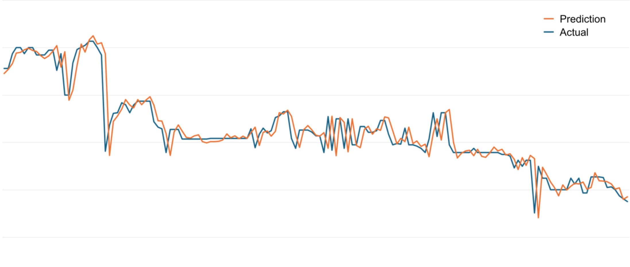
The task of predicting one minute into the future clearly involves too much noise. So, I repurposed the model to predict the mean average of the next r minutes of closing prices. I also added a predicted standard deviation as a second output of the model which was removed later as, perhaps tellingly, it wasn't able to converge or display a meaningful spread.
Loss logic

loss_mean = mse(pred_mean, mean_future - current) * alpha_mean
loss_stdev = mse(pred_stdev, future_stdev) * alpha_stdev
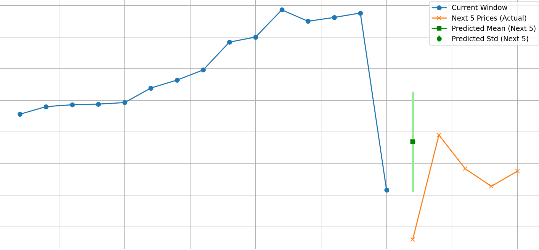
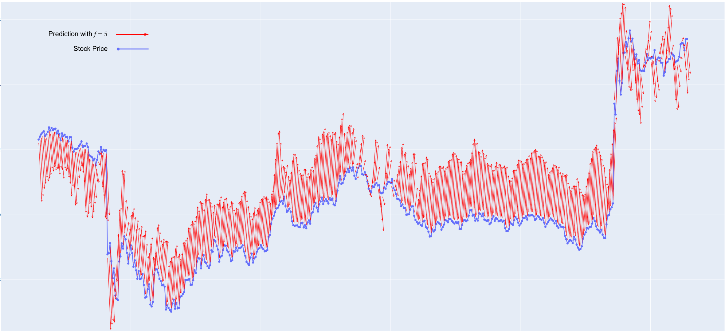
The model worked best at r = 5, achieving at best 50.5% sign accuracy after several hours of training.
After 600 trials trading within random 120-minute sessions of NVDA stock using the script below, it had a mean final portfolio of $10003.42, with a standard deviation of $12.30.
This barely beats the market and has nowhere near the reliability of even a simple moving average crossover.
The model had a major bias towards predicting an increase (over 70% of predictions > 0), possibly reflecting the enormous inflation of NVDA stock prices between 2023 and 2024. Trying different stocks over different periods confirmed this. When properly trained with low learning rate over many hundreds of epochs, the model converged towards predicting the same increase/decrease every time, to the point where it was unable to function with the simulation script as it either never bought or bought every single tick until it ran out of cash.
This could be optimised with a more advanced simulation, for example trading different numbers of shares based on the model's prediction, but the model itself needed the most focus.
Trading simulation

model.eval()

bt = 0.8
st = -0.8

cash = 10000.0
shares = 0.0

step = 1
selected_indices = list(range(0, min(len(dataset), num_samples), step))

for idx in selected_indices:
    X, y = dataset[idx]
    X = X.unsqueeze(0).to(device)
    preds = model(X).squeeze(0).cpu().numpy()
    pred = target_scaler.inverse_transform(preds.reshape(-1, 1)).flatten()
    actual = target_scaler.inverse_transform(y.unsqueeze(0).numpy().reshape(-1, 1)).flatten()

    predictions.append(pred)
    actuals.append(actual)
    indices.append(idx + dataset.window_size)

    current_close = dataset.close[idx + dataset.window_size]
    d = pred[0] * pred_scale
    predicted_next = d + current_close

    if d > bt and cash >= current_close:
        shares += 1
        cash -= current_close
        buy_signals.append(idx + dataset.window_size)
    elif d < st and shares >= 1:
        shares -= 1
        cash += current_close
        sell_signals.append(idx + dataset.window_size)


final_value = cash + shares * current_close
Supplementing with technical indicators
Initially, I tried several features including a few candlestick patterns.
feature_cols = ["close", "open", "high", "low", "volume",
                "rsi", "macd_line", "macd_sig",
                "boll_mid", "boll_up", "boll_low",
                "stoch_k", "stoch_d", "sma_10",
                "sma_50", "obv", "mfi", "hammer",
                "doji", "engulfing",
                "close_lag_1", "close_lag_2", "close_lag_3",
                "close_lag_4", "close_lag_5"]
I incorporated a diversity loss in an attempt to steer the model away from getting stuck. Gradient clipping also seemed to help.
Diversity loss and sign tracking

similarity = torch.matmul(summed_outputs_normalized, summed_outputs_normalized.T)
mask = torch.eye(similarity.size(0), device=device).bool()
diversity_loss = similarity[~mask].mean()

total_loss = pred_loss + diversity_weight * diversity_loss

optimizer.zero_grad()
total_loss.backward()
optimizer.step()

total_train_loss += pred_loss.item()

pred_mean = predictions[:, 0]
target_mean = target_tensor[:, 0]
pred_sign = torch.sign(pred_mean)
target_sign = torch.sign(target_mean)
nonzero_mask = (target_sign != 0)
correct_sign = (pred_sign == target_sign) & nonzero_mask
train_correct += correct_sign.sum().item()
train_total_nonzero += nonzero_mask.sum().item()
However, the model converged to a hybrid of the indicators - seemingly a cross between a moving average and a bollinger band. Perhaps this suggests that they have some predictive value, but most likely the complete opposite - I had succeeded in keeping the model away from the same predictions every time, and there was now nothing meaningful to converge to.
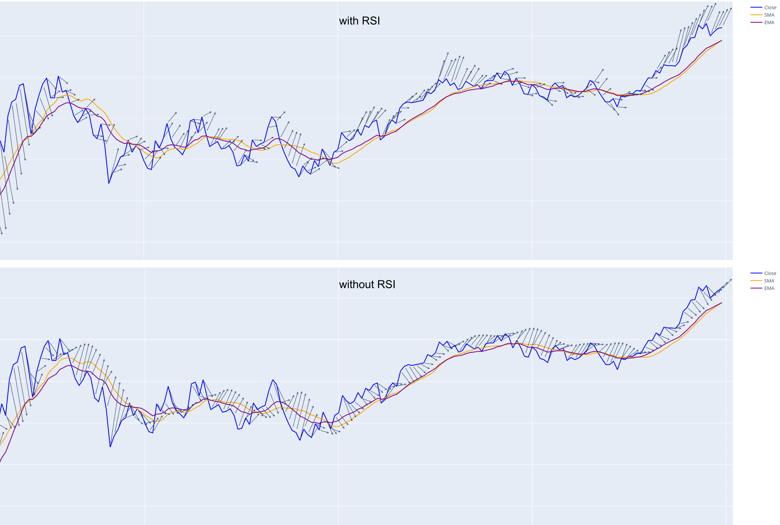
For consistency, all windows and spans of technical indicators were kept the same. With span s > 4r, the indicators provided little use as they were too slow to react. Ideally they would have an adaptive time frame, but the model would not converge properly with this.
Removing the indicators one by one revealed the RSI to be the most influential. With r = 5, the model was able to achieve at least 53% accuracy for predicting the direction. This was massively weighed down by large price shifts, where it repeatedly predicted against the current market momentum. Again, an adaptive time frame would help with this.
The simplified LSTM

def compute_rsi(s, period=14):
    d = s.diff()
    g = d.clip(lower=0)
    l = -d.clip(upper=0)
    ag = g.rolling(window=period).mean()
    al = l.rolling(window=period).mean()
    rs = ag / al
    return 100 - (100 / (1 + rs))

def compute_sma(s, window=14):
    return s.rolling(window=window).mean()

def compute_ema(s, span=14):
    return s.ewm(span=span, adjust=False).mean()

df = pd.read_csv('data/NVDA_1min_467k.csv')
df['rsi'] = compute_rsi(df['close'])
df['sma'] = compute_sma(df['close'])
df['ema'] = compute_ema(df['close'])
df = df.dropna().reset_index(drop=True)
r = 5
seq_length = 60
features = ['close','rsi','sma','ema']
arr = df[features].values
Xs = []
ys = []
for i in range(seq_length, len(arr)-r+1):
    seq = arr[i-seq_length:i]
    fut = arr[i:i+r,0]
    tgt = np.mean(fut)
    Xs.append(seq)
    ys.append(tgt)
Xs = np.array(Xs)
ys = np.array(ys)
split = int(len(Xs)*0.8)
X_train = Xs[:split]
y_train_orig = ys[:split]
X_test = Xs[split:]
y_test_orig = ys[split:]
train_mean = X_train.mean(axis=(0,1))
train_std = X_train.std(axis=(0,1))
X_train_norm = (X_train - train_mean) / train_std
X_test_norm = (X_test - train_mean) / train_std
tgt_mean = y_train_orig.mean()
tgt_std = y_train_orig.std()
y_train_norm = (y_train_orig - tgt_mean) / tgt_std
y_test_norm = (y_test_orig - tgt_mean) / tgt_std
X_train_tensor = torch.tensor(X_train_norm, dtype=torch.float32).to(device)
y_train_tensor = torch.tensor(y_train_norm, dtype=torch.float32).unsqueeze(1).to(device)
X_test_tensor = torch.tensor(X_test_norm, dtype=torch.float32).to(device)
y_test_tensor = torch.tensor(y_test_norm, dtype=torch.float32).unsqueeze(1).to(device)

class LSTMNet(nn.Module):
    def __init__(self, inp):
        super(LSTMNet, self).__init__()
        self.l1 = nn.LSTM(inp, 512, batch_first=True)
        self.l2 = nn.LSTM(512, 256, batch_first=True)
        self.l3 = nn.LSTM(256, 32, batch_first=True)
        self.l4 = nn.LSTM(32, 16, batch_first=True)
        self.l5 = nn.LSTM(16, 1, batch_first=True)
    def forward(self, x):
        x, _ = self.l1(x)
        x, _ = self.l2(x)
        x, _ = self.l3(x)
        x, _ = self.l4(x)
        x, _ = self.l5(x)
        x = x[:, -1, :]
        return x

model = LSTMNet(len(features)).to(device)
opt = optim.Adam(model.parameters(), lr=0.0001)
loss_fn = nn.MSELoss()
bs = 256
eps = 200
for e in range(eps):
    epoch_loss = 0.0
    batches = 0
    perm = torch.randperm(X_train_tensor.size(0))
    for i in range(0, X_train_tensor.size(0), bs):
        idx = perm[i:i+bs]
        bx = X_train_tensor[idx]
        by = y_train_tensor[idx]
        opt.zero_grad()
        out = model(bx)
        loss = loss_fn(out, by)
        loss.backward()
        opt.step()
        epoch_loss += loss.item()
        batches += 1
    model.eval()
    with torch.no_grad():
        preds_train_norm = model(X_train_tensor).squeeze().cpu().numpy()
        preds_train = preds_train_norm * tgt_std + tgt_mean
    print(f"Episode {e+1}/{eps} - Loss: {epoch_loss / batches:.6f}")
    model.train()
There may be some experimentation to be done with this result, such as building a trading strategy based on the output. The model does add some value to the standalone indicators as it has an actual prediction rather than a vague outlook. It can also be specifically trained to an individual stock.
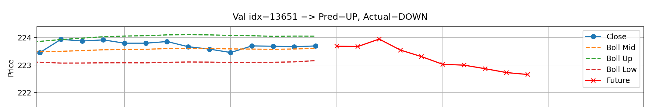
Predicting the direction of price change
When building the trading simulations themselves, I found that the most useful information was a simple binary UP/DOWN as in a practical sense the decision comes down to buying, selling or holding.
So I built a very similar LSTM network to do exactly this. Admittedly, there was no architectural difference as it simply reported UP, DOWN, UNSURE based on thresholds on the final neuron. The difference came in the training, where it was given a target of 1.000 for an increase, -1.000 for a decrease and 0.000 for no single-direction change.
Loss logic

target = torch.sign(avg_future) if torch.abs(avg_future) > 0.8 else 0.0
snapped_pred = (0.0 if torch.abs(pred) < 0.8 else torch.sign(pred))
loss = 0.0 if snapped_pred == target else (0.6 if snapped_pred == 0 else 1.0)
It was difficult to get network to predict anything other than the same value each time. I wanted to incentivise choosing UNSURE rather than a confident UP or DOWN, hence the 0.6.
Stage 3: Pattern networks
The idea for the pattern network structure was loosely inspired by convolutional networks. The basic idea is that several small dense networks are iterated through every combination of the close prices in the input time series. Each value Sn(X) represents the summed value of the nth pattern network's outputs, Pn :
The weighting function favours more recent combinations - this helps to diversify the model's predictions by increasing the relevance of recent patterns. The maximum index m is the most recent index in the combination, and α is the context window size.
ca is the ath combination of the set of k elements from X which has l total elements. A span limit λ was also added to improve the relevance of the patterns in the data - and also to cut down on the value R, which can be calculated by the following:
The structure and training process of the network is outlined below.

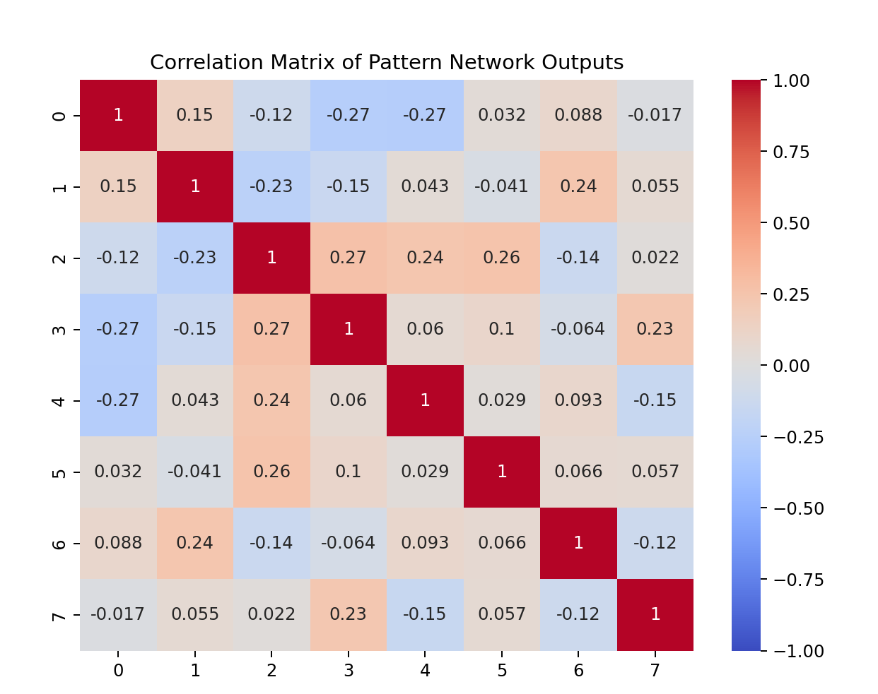
Pattern decorrelation loss

centered = aggregated_outputs - aggregated_outputs.mean(dim=0, keepdim=True)
cov = (centered.t() @ centered) / (centered.size(0) - 1)
diag = cov.diag()
denom = torch.sqrt(torch.outer(diag, diag)).clamp(min=eps)
correlation = cov / denom
I = torch.eye(correlation.size(0), device=correlation.device)
loss = ((correlation - I)**2).sum()
return loss
After initially training the pattern networks, the correlation matrix showed that it was possible to get several somewhat unique interpretations of the data. The main network was harder to train, but eventually produced somewhat workable results. Simply taking the gradient of the main network prediction over time and finding its crossover point with the axis, and buying and selling at that point when the prediction is positive or negative is suitable for a profitable trading strategy.
This is still in development, and the article will be updated with progress.